Timestral: A 209M-Parameter Forecaster That Ranks First on Three Benchmarks

Mistral has released Timestral, its first family of time-series foundation models. The headline number is the size: the largest model has 209M parameters and ranks first on GIFT-Eval, TIME and fev-bench, beating the previous state of the art with about two-thirds of its parameter count. The family spans four sizes, 5M, 28M, 123M and 209M, and the smaller ones are where it gets practical.

Where the benchmark numbers stand

Among pre-trained, zero-shot models, the 209M checkpoint ranks first on all five metrics the team reports across the three benchmarks: GIFT-Eval GMean WQL and GMean MASE, TIME GMean CRPS and GMean MASE, and the SQL skill score on fev-bench. Those results come from a single checkpoint with no ensembling, which matters if you've ever compared a headline score against a tuned ensemble. The results have been submitted to the GIFT-Eval and TIME leaderboards.

One caveat for anyone reading the charts in the announcement: the bar graphs use truncated axes. The GIFT-Eval WQL axis starts at 0.44, the MASE axis at 0.65, the TIME CRPS axis at 0.515 and the fev-bench skill axis at 44%. Bar length therefore doesn't track the score ratio. Read the labels, not the bar lengths, and check the leaderboards for exact values.

The team also claims that the family sits on the Pareto front of accuracy versus model size, meaning no public model forecasts better at any given size. Two comparisons stand out. The 28M model beats Chronos-2, which is roughly four times larger, on GIFT-Eval and TIME. The 209M model beats TimesFM-3 and Falcon-2.0 while carrying fewer parameters.

Speed on ordinary hardware

Timestral doesn't need a GPU at inference. On a standard server CPU with 8 threads, forecasting one day ahead from three weeks of 15-minute history takes 17 ms with the 5M model and 113 ms with the 209M model. The middle sizes make a clear trade. The 28M model is 3.6 times faster than the 209M, and the 123M model lands within 0.2% of the 209M score at about three-quarters of its latency.

That's the number that will matter most to teams running forecasts across thousands of series. Latency that's measured in milliseconds per series, on CPUs already in the rack, changes what's economical to forecast. You can afford to forecast everything rather than sampling the important assets.

Why pre-training matters for forecasting

Classical tools like ARIMA and linear regression are usually fitted to one series and learn only from that series' history. Deep models such as PatchTST can capture nonlinear patterns across many related series, but they're typically trained from scratch on each dataset, so what they learn stays inside that dataset. Foundation models change the setup. Trained on a large and varied corpus, they learn patterns that transfer, which lets them forecast zero-shot on series they've never seen. That's most useful where local history is thin.

What's under the hood

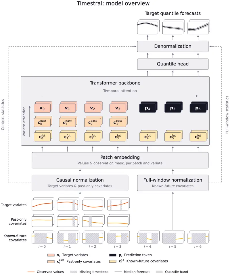
Timestral combines four ideas, and the technical report covers each in detail.

Decoupled Horizon Forecasting (DHF). Causal decoders trained with contiguous patch masking, as in Toto 2.0 and TimesFM-3, hide the values they must predict. Those hidden values look like missing data, and they're lost as context for later forecasts. DHF separates the two jobs. The full history stays in the sequence, and learned forecast tokens read the history before them. Every observed value serves as both target and context, true gaps remain flagged as missing, and training horizon length and missing-data augmentation can be tuned independently.

Covariate-aware attention. Each input series gets a role: target variate, past-only covariate or known-future covariate. Known-future covariates are visible across the whole window, while targets stay causal, and information flows only from covariates into targets. A holiday calendar or weather forecast can inform the model without leaking a target's own future values.

Synthetic-first data. Most of the training data is synthetic. The team generated univariate processes with trends, seasonality and varied noise, then used a multivariate synthesizer to introduce nonlinear dependencies between them. Synthetic data also gives you a clean way to build a test set the model has never seen, which the team points to when discussing backtests.

Two-stage training. The model is pre-trained at scale on purely synthetic data with a context of 8,192 steps, then post-trained on a mix of real and synthetic data with a context 4x longer. The objective is a pinball loss over 21 quantiles, a discrete approximation of CRPS. That's why the output is a distribution rather than a single point.

Where it fits in an industrial stack

The announcement's example is a plant with thousands of sensors. Timestral addresses four things that single-series models handle poorly. It models related series jointly, so a pump's vibration, temperature and pressure can inform each other rather than being forecast in isolation. It outputs a full set of quantiles, so alert thresholds can reflect actual uncertainty. It accepts categorical covariates such as machine state or day of the week as categories rather than forced numeric codes. And it conditions on known-future drivers like production schedules and planned shutdowns, so a scheduled load increase registers as expected rather than as an anomaly.

Mistral also pitches Timestral as a component in agentic workflows. In the plant scenario, the model runs continuously on sensor streams and flags anomalies. When it flags a pump, an agent embeds the signals and searches past sensor data for similar failures. Sub-agents then pull in maintenance records, shift logs, manuals, work orders and readings from related equipment to run a root cause analysis. The output is a draft diagnosis with supporting evidence and next steps. My read is that the forecasting model is the easy part to evaluate here. The harder question is how well the retrieval and diagnosis steps hold up, and the announcement doesn't provide numbers for those.

Adapting it to your data

Public benchmarks measure general performance, and production data can differ in structure and behaviour. Markets change regime, equipment degrades and demand patterns move. Teams in this position typically care less about leaderboard rank than about how fast a model can be adapted and retrained as the distribution shifts.

Timestral is available through Mistral Forge, which uses the same training pipeline as Mistral's language models. Forge supports zero-shot inference out of the box, architectural extensions such as domain-specific covariates, and fine-tuning on proprietary data while aiming to preserve general performance. Teams also get control over the training mix, can replay pre-training data and can generate synthetic samples that reflect their domain. The full pipeline can be deployed on-premises, in a VPC or in air-gapped environments.

Specs and access

Spec	Timestral
Type	Time-series foundation model (TSFM)
Parameters	5M, 28M, 123M and 209M
Context length	32,768 time steps
Output	Probabilistic forecasts, 21 quantiles
Inputs	Multivariate targets, past-only and known-future covariates
Deployment	On-prem, VPC or air-gapped
Licence	Modified MIT

The weights are on Hugging Face, the code is in the GitHub repository, and the full results and methods are in the technical report. Run it on your own series before trusting the leaderboard. Timestral's real test is whether its zero-shot accuracy and CPU latency hold up on your data, and whether the 5M and 28M models hold their ground where you can't afford anything larger.